Sanika Khadkikar

For my research, I primarily use gravitational wave signals to estimate the source parameters of binary mergers observed by LIGO. Although most of my previous work has focused on forecasting binary neutron star observations, I have had very limited interaction with real detector data. To address this, I recently began volunteering as an analyst for actual gravitational wave events. This post is a primer on the pre-processing steps applied to the raw data before it is passed to the Bayesian inference pipeline for parameter estimation.

Gravitational wave signals in their raw form must go through several stages of processing before they are suitable for inference. These steps help clean the signal and prepare it for extracting meaningful physics. One of the first and most essential steps is whitening.

Detector data includes not only the gravitational wave signal but also significant noise from various sources, such as seismic motion, thermal fluctuations, photon shot noise, and human activity. This noise varies with frequency, and its distribution is described by the power spectral density (PSD), which is estimated using data that does not contain any astrophysical signal.

In the case of LIGO, the PSD typically shows much higher noise at low frequencies (below about 20 Hz) and at very high frequencies (above about 1000 Hz). Even within the most sensitive frequency band, the noise is not uniform. To ensure all frequency components are treated equally in the analysis, we flatten the noise spectrum by whitening the data. This process divides the signal by the square root of the PSD.

The reason we whiten the data is not because nature prefers flat noise spectra, but because the downstream analysis tools require the noise to be white and Gaussian. This means the noise must have zero mean, unit variance, and no frequency preference. When noise power varies across frequencies, it is called colored noise. Colored noise makes some frequency bands noisier than others, which interferes with our ability to recover accurate source parameters. Whitening removes this issue and allows the gravitational wave signal to appear as sharp features against a uniform background.

For the loudest signal ever seen with LIGO (GW230814), I will now describe the code used for this step.

import matplotlib.pyplot as plt
import gwpy.timeseries

trigger_time = 1376089759.8100667
tstart = trigger_time - 500
tend = trigger_time + 10

l1_strain = TimeSeries.get(channel='L1:GDS-CALIB_STRAIN_CLEAN', start=tstart, end=tend)
plt.figure(figsize=(15,3))
plt.plot(l1_strain)
plt.axvline(trigger_time, color='red')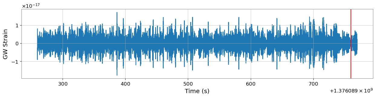

Figure: Raw LIGO strain data centered around the trigger time.

Just by inspecting the data shown above, it is impossible to discern anything about the signal. The signal's location is not even visually obvious. To make the features of the data more interpretable, the data must first be whitened. Whitening flattens the noise spectrum, which requires an accurate estimate of the PSD.

The most basic approach to estimating the PSD is the Periodogram:

$$PSD_{\text{Periodogram}}(f) = \frac{1}{T} |\mathcal{F}(h(t))|^2$$

This method is highly sensitive to fluctuations because it is computed from just one realization of the data. A more robust alternative is the Welch method, which splits the data into $K$ overlapping segments, windows each segment, and averages (or takes the median of) the power spectra:

$$PSD_{\text{Welch}}(f) = \frac{1}{K} \sum_{k=1}^K |\mathcal{F}(h_k(t))|^2$$

In GW analyses, the median is preferred over the mean because it is less sensitive to glitches and more representative of the stationary noise floor.

detectors = ['L1']
channels = {'L1': 'L1:GDS-CALIB_STRAIN_CLEAN'}
start_time = trigger_time - 4
duration = 6
ifos = bilby.gw.detector.InterferometerList([])

psd_gps_start_time = start_time - 512
psd_gps_end_time = psd_gps_start_time + 256

for detector in detectors:
    ifo = bilby.gw.detector.get_empty_interferometer(detector)
    ifo.minimum_frequency = 20
    ifo.maximum_frequency = 1024
    ifo.set_strain_data_from_channel_name(
        channel=channels[detector],
        sampling_frequency=4096,
        duration=duration,
        start_time=start_time
    )
    ts = TimeSeries.get(
        channel=channels[detector],
        start=psd_gps_start_time,
        end=psd_gps_end_time
    )
    ts = ts.highpass(20)
    psd = ts.psd(fftlength=16, overlap=8, method='median')
    ifo.power_spectral_density = bilby.gw.detector.PowerSpectralDensity(
        frequency_array=psd.frequencies.value,
        psd_array=psd.value
    )

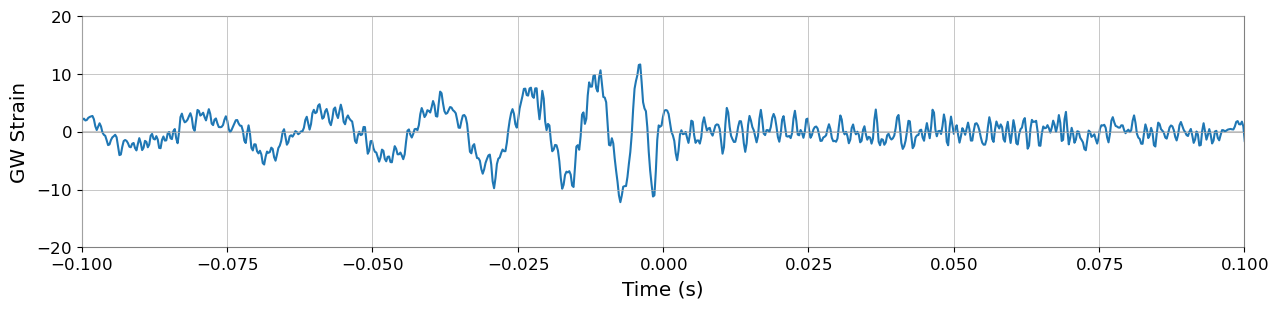
Figure: The whitened data using median Welch PSD. The signal is now clearly visible.

frequency_window_factor = (np.sum(ifo.frequency_mask) / len(ifo.frequency_mask))
whitened_time_series = (np.fft.irfft(ifo.whitened_frequency_domain_strain) *
                        np.sqrt(np.sum(ifo.frequency_mask)) / frequency_window_factor)

plt.figure(figsize=(15, 3))
plt.plot(ifo.time_array - trigger_time, whitened_time_series)
plt.ylim(-20, 20)
plt.xlim(-0.1, 0.1)

This worked beautifully for GW230814, but failed for S240601co — a lower SNR (~8) event. Two reasons:

1. The signal is intrinsically weaker, so harder to see even after whitening.
2. A glitch occurred a few seconds before the event, contaminating the data.

To spot such glitches, Q-scans are useful. These are time-frequency plots made by fitting wavelets of varying quality factors:

$$Q = \frac{f_0}{\Delta f}$$

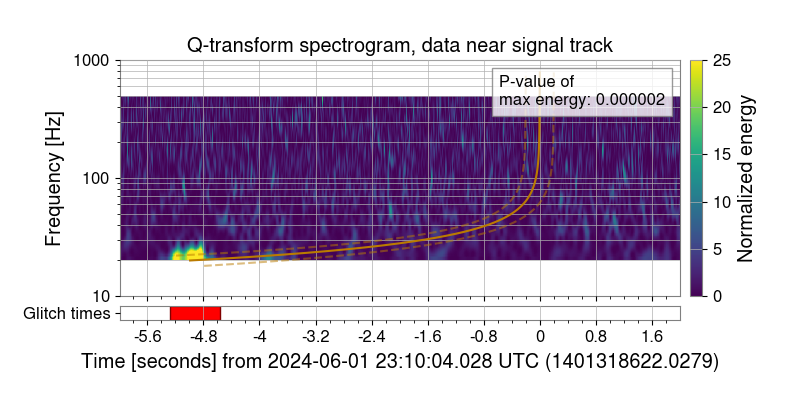
Figure: Q-scan showing a glitch near -5 seconds before S240601co.

Using wavelet-based subtraction (e.g., via BayesWave), such glitches can be modeled and removed.

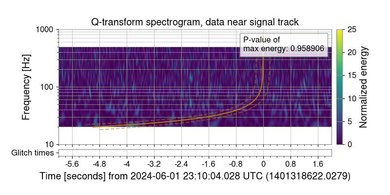
Figure: Q-scan after glitch subtraction using BayesWave. Clean and glitch-free!

Initially, Welch PSD estimation with 16-second segments failed because the data was non-stationary. Reducing the segment length to 4 seconds made it work. This hands-on process really taught me how sensitive and nuanced GW data analysis is. It was fun doing this :) Cheers!